Dimensionality Reduction Techniques in Machine Learning: using Python


Introduction:
Hi folks, here in this post we will see different types of Dimensionality Reduction techniques used in machine learning using python. In Machine Learning, it's common to work on more than a thousand features. In that case, it becomes difficult to analyze thousands of features and extract patterns or insights from them and some algorithms don't work well with lots of features so in that case, we can use the concept of dimensionality reduction, it is used to reduce the number of features from the dataset which is not much important for our machine learning task without losing the model's performance.
Why Dimensionality Reduction:
It's very challenging and time-consuming to work on thousands of features as well as difficult to visualize data in higher dimensions. Sometimes we face Curse of Dimensionality problem when we have a high dimensional dataset. Some algorithms do not work well with high-dimensional data and it reduces the model's performance. By doing Dimensionality Reduction we can take care of multicollinearity by removing redundant features. For example, If two features are highly correlated with each other and if we train the model with both features then the performance of the model might get decreases so in that case it makes to remove one feature from the dataset.
Dimensionality reduction can be divided into two different types:
Feature Selection: In this technique we will select the most relevant features from the original dataset.
Dimensionality Reduction: In this technique we will find a new set of features and each new feature is constructed from the original dataset.
Feature Selection techniques:
- Missing Value Ratio.
- High Correlation filter.
- Low Variance Filter.
- Random Forest.
- Forward Feature Selection.
- Backward Feature Elimination.
Dimensionality Reduction techniques:
- Factor Analysis.
- Principal Component Analysis (PCA).
- Linear discriminant analysis (LDA).
- t-SNE.
- UMAP.
Feature Selection Techniques:
For Feature Selection Techniques we will use House price prediction dataset.
Import required libraries and load CSV file.
import pandas as pd
import numpy as np
import matplotlib.pyplot as plt
data = pd.read_csv("data.csv") # path to csv file
data.columns
#['date', 'price', 'bedrooms', 'bathrooms', 'sqft_living', 'sqft_lot',
#       'floors', 'waterfront', 'view', 'condition', 'sqft_above',
#       'sqft_basement', 'yr_built', 'yr_renovated', 'street', 'city',
#       'statezip', 'country']
# Total we have 17 features and 'price' is our target variable
1. Missing Value Ratio: Suppose we have a dataset and we found few missing values in our dataset. The first step will be to fill the missing values with the proper imputation technique. But what if we have too many missing values(like more than 50% are missing) in one of our features. In that case, it makes sense to remove the entire feature rather than filling missing value as it does not carries much information. So Missing Value Ratio is a technique to remove the feature completely from the dataset if it has too many missing values. We set a threshold value, and if the percentage of missing value in any feature is greater than the threshold then we will drop that particular feature.
(data.isnull().sum()/len(data))*100 # percentage of missing value in our dataset
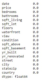 Here in the above example, we didn't find any missing value.
2. High Correlation filter: If two features are highly correlated with each other then it means they carry similar information and using both features will decrease the model's performance. So to overcome this situation, we will use the technique called the High Correlation filter. In this technique, we will calculate the correlation between numeric features and if the correlation value crosses a threshold value then we will drop one of the features from our dataset. Generally, we keep those features that show a high correlation with the target variable.
X_train=data.drop(['date','price'], axis=1) # we have dropped "data" and "price" is our target variable
X_train.corr()
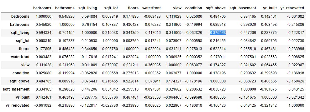 Here in the above example, it looks like sqft_living is highly correlated with sqft_above. So we can drop any one of these features(Before dropping any feature, we should check the correlation of feature with target variable)
3. Low Variance Filter: Consider we have a feature in our dataset and it has only one unique value. For Example, let's say we have a feature called "country" and it has only one unique value "India". And if we use this feature in our training, then it won't improve our model's performance because this feature will have zero variance. In the Low Variance Filter, we will calculate variance for each feature then drop the feature which has low variance as compared to other features in our dataset.
X_train['country'].value_counts()
# country column has only one value "USA"
Here in the above example, for the "country" column, it has only one unique value. So we can drop this features as it does not add any value in our prediction.
4. Random Forest: Random Forest is one of the important algorithm in Machine Learning and it is a widely used algorithm for feature selection as well. It comes with inbuilt feature importance as it calculates important features at every node/step.
#https://scikit-learn.org/stable/modules/generated/sklearn.ensemble.RandomForestRegressor.html
from sklearn.ensemble import RandomForestRegressor
from sklearn import preprocessing
X_train = data.drop(['date','street','country','price'], axis=1)
Y_train = data['price']

# statezip has "WA 12334" values so we will preprocess and remove first 3 chars to convert it into numeric
X_train['statezip'] = X_train.apply(lambda row: row['statezip'][3:], axis=1)

# we will use label encoding to convery city column into numeric feature
city_le = preprocessing.LabelEncoder().fit_transform(X_train['city'])
X_train['city'] = city_le

model = RandomForestRegressor(random_state=1, max_depth=10)
model.fit(X_train,Y_train)

###################################################

features = X_train.columns
importances = model.feature_importances_
indices = np.argsort(importances)
plt.grid()
plt.title('Feature Importance')
plt.barh(range(len(indices)), importances[indices], align='center')
plt.yticks(range(len(indices)), [features[i] for i in indices])
plt.show()
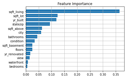
The above graph shows feature importance using Random Forest, we can choose the important features from the above graph and ignore the remaining features.
5. Forward Feature Selection: A Forward Feature Selection is an iterative method in which we start with one feature. In each iteration, we will add one feature at a time and train our model. And the feature which gives the highest improvement in performance is retained. Then repeat this process until no significant improvement in the model's performance is seen.
#https://scikit-learn.org/stable/modules/generated/sklearn.feature_selection.SequentialFeatureSelector.html
from sklearn.feature_selection import SequentialFeatureSelector
from sklearn.linear_model import LinearRegression
lreg = LinearRegression()
sfs = SequentialFeatureSelector(lreg, n_features_to_select=10,direction='forward') # Here we are passing "10" to get top 10 features
result = sfs.fit_transform(X_train,Y_train)
selecte_features = sfs.get_support()

cols = list(X_train.columns)
features = []
for i in range(len(selecte_features)):
    if selecte_features[i] == True:
        features.append(cols[i])
print(features)
# Here are the top 8 features for Forward features selection
# output = ['bedrooms', 'bathrooms', 'sqft_living', 'sqft_lot', 'floors', 'waterfront', 'view', 'condition', 'yr_built', 'city']
Above example giving the top 10 features using the Forward Feature Selection technique.
6. Backward Feature Elimination: A Backward Feature Elimination is the reverse process of Forward Feature Selection. In Backward Feature Elimination, we will start with all features and train our model and then calculate the performance of our model. After that, we will remove one feature at a time and train the model to see the performance. Now we will identify the feature that produces very little change in the model's performance after removal, then we will drop that feature. We will repeat this until no feature can drop from the remaining features.
#https://scikit-learn.org/stable/modules/generated/sklearn.feature_selection.SequentialFeatureSelector.html
from sklearn.feature_selection import SequentialFeatureSelector
from sklearn.linear_model import LinearRegression
lreg = LinearRegression()
sfs = SequentialFeatureSelector(lreg, n_features_to_select=10,direction='backward') # Here we are passing "10" to get top 10 features
result = sfs.fit_transform(X_train,Y_train)
selecte_features = sfs.get_support()

cols = list(X_train.columns)
features = []
for i in range(len(selecte_features)):
    if selecte_features[i] == True:
        features.append(cols[i])
print(features)
# Here are the top 8 features for Forward feature selection
# output = ['bedrooms', 'bathrooms', 'sqft_living', 'sqft_lot', 'floors', 'waterfront', 'view', 'yr_built', 'city', 'statezip']
Above example giving the top 10 features using the Backward Feature Elimination technique.
Dimensionality Reduction Techniques:
To see the importance of Dimensionality Reduction Techniques, we will use the Digit Recognizer(MNIST) dataset.
It has a total of 784(represents 28 * 28 image) features and 1 target column(it has 0 to 9 class labels).
Import required libraries and load CSV file.
import pandas as pd
import numpy as np
import seaborn as sn
import matplotlib.pyplot as plt
data = pd.read_csv("train.csv") # path to csv file
X_train = data.drop("label",axis=1)
Y_train = data['label']
1. Factor Analysis: Factor analysis is one of the unsupervised machine learning algorithm which is used for dimensionality reduction. This technique extracts maximum common variance from all features and puts them into a common group. For Example, let's say we have two features "area_of_house" and "price_of_house", these two features are highly correlated with each other as if area_of_house is increasing then prise_of_house will also increase and vise versa. So Factor Analysis will group the features in such a way that all the features in one group will have a high correlation among themselves and a low correlation with other groups. Each group is known as Factor.
#https://scikit-learn.org/stable/modules/generated/sklearn.decomposition.FactorAnalysis.html
from sklearn.decomposition import FactorAnalysis
fa = FactorAnalysis(n_components = 2)
fa_result = fa.fit_transform(X_train.values)
factor_analysis_data = np.vstack((fa_result.T, Y_train)).T
fa_df = pd.DataFrame(data=factor_analysis_data, columns=("1st_factor", "2nd_factor", "label"))
sn.FacetGrid(fa_df, hue="label", size=6).map(plt.scatter, '1st_factor', '2nd_factor').add_legend()
plt.grid()
plt.show()
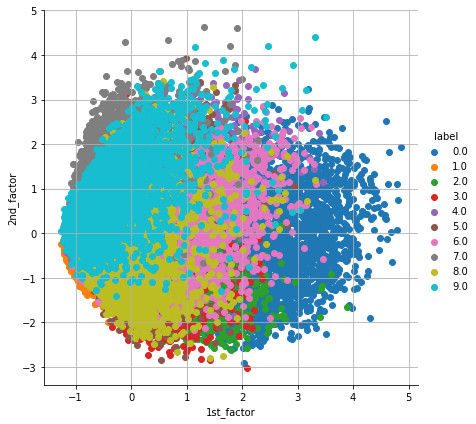 The above graph shows two decomposed factors for the given dataset. The X-axis and Y-axis represent the value of each factor.
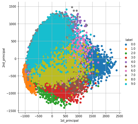
2. Principal Component Analysis (PCA): PCA is one of the important and widely used unsupervised technique for dimensionality reduction technique. PCA generates new features from the given dataset and each feature generated from PCA are known as Principal Components. PCA extracts components in such a way that the first component explains maximum variance, the second component tries to explain the remaining variance, and so on.
#https://scikit-learn.org/stable/modules/generated/sklearn.decomposition.PCA.html
from sklearn.decomposition import PCA
pca = PCA(n_components=2)
pca_data = pca.fit_transform(X_train.values)
pca_data = np.vstack((pca_data.T, Y_train)).T # Take transpose of result so we can convert it into dataframe for visualization

pca_df = pd.DataFrame(data=pca_data, columns=("1st_principal", "2nd_principal", "label"))
sn.FacetGrid(pca_df, hue="label", size=6).map(plt.scatter, '1st_principal', '2nd_principal').add_legend()
plt.grid()
plt.show()
Let's see cumulative variance explained by PCA so we can see how many components explain more than 95% variance.
#https://scikit-learn.org/stable/modules/generated/sklearn.decomposition.PCA.html
from sklearn.decomposition import PCA
pca = PCA(n_components=784)
pca_data = pca.fit_transform(X_train.values)
percentage_var_explained = pca.explained_variance_ / np.sum(pca.explained_variance_);
cumulative_var_explained = np.cumsum(percentage_var_explained)

plt.grid()
plt.plot(cumulative_var_explained, linewidth=2)
plt.xlabel('Number of components')
plt.ylabel('Cumulative variance explained')
plt.show()
print(cumulative_var_explained[300]) # top 300 components explains more than 0.9864525611439835 (98%) of varience
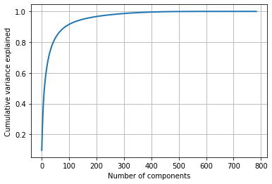 From the above graph, we can say that the top 300 components explaining around 98% of the variance.
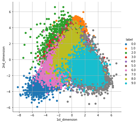
3. Linear discriminant analysis (LDA): A Linear discriminant analysis (LDA) is one of the popular supervised algorithm for Dimensionality Reduction which uses all features from the given dataset to create new features in such a way that it minimizes the variance and maximizes the distance between the means of classes.
#https://scikit-learn.org/stable/modules/generated/sklearn.discriminant_analysis.LinearDiscriminantAnalysis.html
from sklearn.discriminant_analysis import LinearDiscriminantAnalysis
lda = LinearDiscriminantAnalysis(n_components=2)
lda_data = lda.fit_transform(X_train.values,Y_train)

lda_data = np.vstack((lda_data.T, Y_train)).T # Take transpose of result so we can convert it into dataframe for visualization

lda_data = pd.DataFrame(data=lda_data, columns=("1st_dimension", "2nd_dimension", "label"))
sn.FacetGrid(lda_data, hue="label", size=6).map(plt.scatter, '1st_dimension', '2nd_dimension').add_legend()
plt.grid()
plt.show()
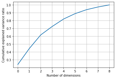
 Let's see the cumulative variance ratio explained by LDA with the below code and graph.
#https://scikit-learn.org/stable/modules/generated/sklearn.discriminant_analysis.LinearDiscriminantAnalysis.html
from sklearn.discriminant_analysis import LinearDiscriminantAnalysis
lda = LinearDiscriminantAnalysis(n_components=9)
lda_data = lda.fit_transform(X_train.values,Y_train)
percentage_var_explained = lda.explained_variance_ratio_ / np.sum(lda.explained_variance_ratio_);
cumulative_var_explained = np.cumsum(percentage_var_explained)

plt.grid()
plt.plot(cumulative_var_explained, linewidth=2)
plt.xlabel('Number of dimensions')
plt.ylabel('Cumulative explained variance ratio')
plt.show()
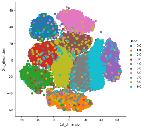
4. t-Distributed Stochastic Neighbor Embedding (t-SNE): t-SNE is one of the widely used unsupervised dimensionality Reduction technique. t-SNE tries to preserve both Local and Global structure of the data. It calculates the similarity between points in both high dimensional as well as in low dimensional space.
#https://scikit-learn.org/stable/modules/generated/sklearn.manifold.TSNE.html
from sklearn.manifold import TSNE
tsne = TSNE(n_components=2, random_state=10) # we should always play with "perplexity" value to get better results.
tsne_data = tsne.fit_transform(X_train.values)

tsne_data = np.vstack((tsne_data.T, Y_train)).T
tsne_df = pd.DataFrame(data=tsne_data, columns=("1st_dimension", "2nd_dimension", "label"))
sn.FacetGrid(tsne_df, hue="label", size=6).map(plt.scatter, '1st_dimension', '2nd_dimension').add_legend()
plt.show()
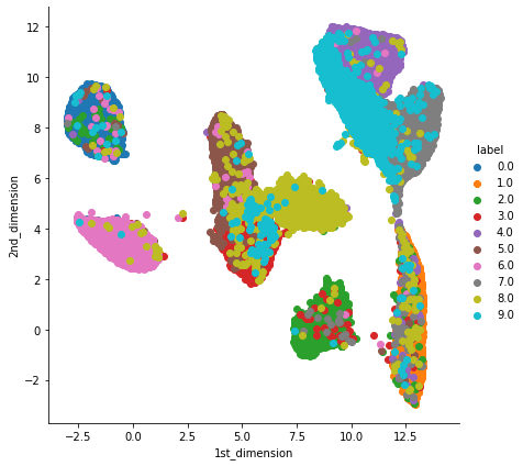
5. UMAP: t-SNE works well but it has some drawbacks like it takes more computation time so we have Uniform Manifold Approximation and Projection(UMAP). UMAP tries to preserves as much of the local structure and more of the global structure as compared to t-SNE with less runtime.
See installation and documentation for UMAP.
!pip install umap-learn # install UMAP library
import umap
umap = umap.UMAP(n_neighbors=50, n_components=2) # we should always play with "n_neighbors" value to get better results.
umap_data = umap.fit_transform(X_train.values)

umap_data = np.vstack((umap_data.T, Y_train)).T
umap_df = pd.DataFrame(data=umap_data, columns=("1st_dimension", "2nd_dimension", "label"))
sn.FacetGrid(umap_df, hue="label", size=6).map(plt.scatter, '1st_dimension', '2nd_dimension').add_legend()
plt.show()
Conclusion:
We have seen various techniques for dimension reduction but when to use which is completely depends on our dataset and we should always try various techniques and select the appropriate technique for our task.