

Introduction:
Hi folks, In this post, we will see how Forward and Backword propagation works in deep learning with code implementation in Julia.
What is Julia:
Python is one of the famous programming language among data science folks as they get an ecosystem with loaded libraries to make the work of data science and analysis faster and more convenient. But Python isn’t fast or convenient enough as most of the libraries are built from other languages such as Java, C, and C++.
To Make faster execution of code, we have Julia. Julia is a high-level and general-purpose language that can be used to write code that is fast to execute and easy to implement for scientific calculations. Julia was built for scientific computing, machine learning, data mining, large-scale linear algebra, distributed and parallel computing.
Please follow the link on how to install and run Julia in Jupiter notebook
Advantages of Julia Language:
- Fast and Secure
- User-friendly syntax
- Package Manager
- Native machine learning libraries
Forward and Backward Propagation in Neural Network:
Forward and Backward propagation is the backbone of the neural network. Forward and backward propagation are the algorithms that can be called the heart of it to converge. The network learns all of its parameters through Forward and Backward propagation.
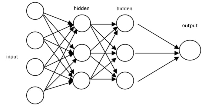
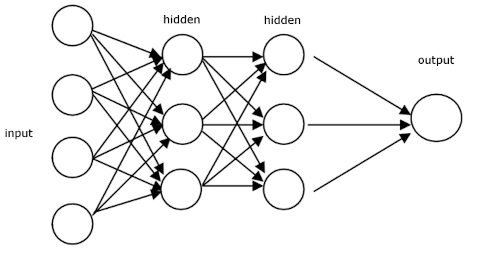
In Forward Propagation, it moves forward from the Input layer (left) to the Output layer (right) with the given input and weights. In FP, we calculate the predicted Y value and Loss function. The process of moving from right to left is called Backward propagation. In Backward Propagation, we reassign the weights to reach the minimized loss function. We reassign the weights by performing partial derivative and chain rule.
Example:
We will see the small example of a neural network and we will implement Forward and Backward Propagation in Julia.
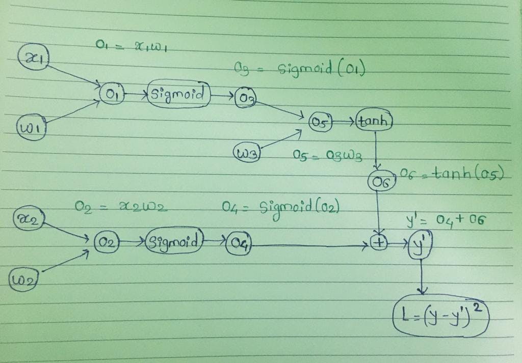
In the example, we have 2 Independent variables (x1 and x2) and 1 dependent variable(y). Here y is continuous(Regression) so we will try to minimize Mean squared error (L) $$MSE = \frac{1}{n} \sum_1^n (Yi - Yi')^2$$ Where, n = number of data points , Y = ground truth, Y' = predicted value
$$Sigmoid(x) = \frac{1}{1+e^-x} , tanh(x) = \frac{e^x - e^-x}{e^x + e^-x}$$ First, we will initialize weights(w) with some random values and then we will perform forward propagation. Once we have done with forward propagation, we will get Y' and Loss.
We will adjust weights so we can minimize the loss function. To adjust weights we will calculate partial derivative of loss(L) with respect to weight(W) with chain rule during backword propagation. $$\frac{\partial L}{\partial w3} = \frac{\partial L}{\partial y'}.\frac{\partial y'}{\partial o6}.\frac{\partial o6}{\partial o5}.\frac{\partial o5}{\partial w3}$$ $$\frac{\partial L}{\partial w2} = \frac{\partial L}{\partial y'}.\frac{\partial y'}{\partial o4}.\frac{\partial o4}{\partial o2}.\frac{\partial o2}{\partial w2}$$ $$\frac{\partial L}{\partial w1} = \frac{\partial L}{\partial y'}.\frac{\partial y'}{\partial o6}.\frac{\partial o6}{\partial o5}.\frac{\partial o5}{\partial o3}.\frac{\partial o3}{\partial 01}.\frac{\partial o1}{\partial w1}$$
After performing the partial derivative and chain rule, we will adjust weights. In our example, we will update weights with 2 different approaches
- Vanilla (SGD)
- Momentum
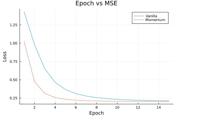 The above graph shows how Loss decreases as the epoch number increases.
Please find the code from GitHub.
Conclusion:
This was my small attempt to demonstrate how we can implement Forward and Backward propagation in Julia. It will help you to write them and understand.